Introduction
BOS or B4 is a software program used to control and operate Protein Crystallography beamlines. It is currently used at beamlines 5.0.1, 5.0.2, 5.0.3, 8.2.1, and 8.2.2 at the Advanced Light Source at Lawrence Berkeley National Laboratory. It was originally based on the SSRL Blu-ice software, so that users from both facilities could move between the two software packages with ease. BOS/B4 can be operated remotely, enabling users to ship samples to the ALS and collect data from their own lab or living room.
Logging in
If you are logging in remotely, you must first connect to the beamline computer using the NX client, as described here. Once you are connected to the beamline computer, open a terminal window on the desktop and type bos or b4. A pop-up will appear asking for a login. Type in your username and password (as supplied by the beamline staff). The data generated during your BOS session will be owned by the user name you login with.
Note: To completely restart the software (both the server and gui) type stopb3 and press return. Wait a moment, and then type startb3 and press return. Wait for the message “server online” then type bos.csh, bos, or b4 to open login window. Note that generally you do not need to use this option.
Mounting a Crystal
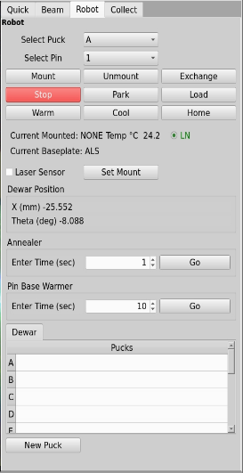
On the Quick or Robot tab to the right of the GUI, select the puck letter and the pin number from the drop-down menu, and then click on Mount. If there is already a pin on the goniometer, you can select Exchange, and this function will first remove the current pin, and then mount the pin you have selected. The mount will take ~20 seconds if the gripper is already cold, and will take ~1 minute if the gripper needs to be cooled first (this happens automatically). For automatic mounting using the Task Manager use the task manager buttons.

Centering a crystal
Click on the Centering tab in the top left of the GUI (picture below).
Click on the sample using the LEFT mouse button. This moves the area clicked beneath the cross hairs and circle, which is the center of rotation. You may have to click a few times to bring the loop into the center of the screen.
You can fine tune your centering using the arrow buttons to the right of the image.
Click on +90 (or -90) to rotate the sample by 90 degrees, and center again.
Click mag 3. This will move the collimator stage in and switch the view to the high-mag camera.
Turn up the microscope backlight if necessary (LED slider is in the Center tab to the right of the GUI).
Click on the sample to center it. Rotate the sample 90 degrees. Center again.
Check the alignment by rotating the sample by 180 degrees. The center of rotation of the loop sample should stay beneath the crosshairs. Please contact staff if you are having trouble centering as an accurate center of rotation is very important.

Getting ready for data collection
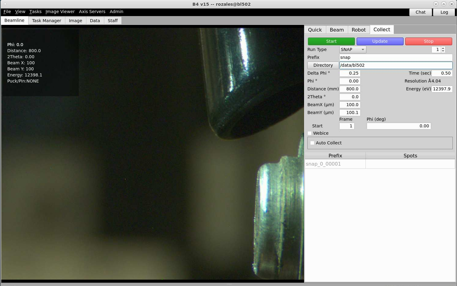
Click either on either the Quick or Collect tab.
Click on the drop down menu where is says “Run Type”. Here you can select SNAP, RUN, VECTOR, RASTER, SCAN.
Set up your data directory: /data/beamline/group/etc… (example, /data/bl502/bcsb/). You can also set up your prefix, but if you wish to just use the prefix defaults, there are for SNAP is snap, RUN and Vector is run, RASTER is raster and SCAN is scan.
Set you your Delta Phi and Time (exposure)
To change the detector distance, type number into the box and press enter (in the picture above, the distance is 750). There is also a box in the collect tab where you can change the distance.
In the collect tab the resolution of the image corresponding to the detector distance you have chosen is shown where is says distance (mm). In the picture below, the resolution at the edge (not the corners) of the detector is 4.04Å. The resolution can also be view in the quick tab below the distance box.
In the collect tab, to move the detector to a 2-theta angle, type a number into the 2Theta box (in the picture below, the 2-theta angle is 0). The detector angle will not change until press enter.
To change the Energy (eV), in the collect tab type a number into the Energy (eV) box and press enter. The example below shows the energy to be 12397.9eV.
The horizontal convergence is normally 2.5 mrad, in the Beam tab (not shown below). You can change this to a smaller value — the result will be a reduction in flux hitting the crystal, and also a reduction in the size of the diffraction spots on the image.
Set the desired collimator size using the BeamX (um) and BeamY (um) settings and press enter. In the picture below it show 100 for both BeamX and BeamY.
Taking a snapshot
Make sure your crystal is centered.
Click on the COLLECT tab in b3.
Click on the 0 in the upper right hand corner. The zero indicates snapshot mode.
Set prefix and directory for the data files. The directory will be created if it does not already exist.
The default MODE is binned (2048×2048), 18 Mb per image (Q315 detector).
Set the detector to desired distance from sample. Standard distances are 150-500 mm.
Set collection time (in seconds), frame number, phi (angle of crystal in degrees), oscillation angle, and energy (in eV).
If you click on UPDATE button in the upper right hand corner the current values (detector distance, energy, angle) are read in. Do not hit UPDATE if you want to enter new values for the snapshot.
Make sure the hutch door is closed and the safety shutter is open.
Click on START to take an image. The dark current is taken if the New Darks box is checked.
After the snapshot is taken, the image will appear in the workspace.
If the adxv viewer is not open, select Adxv Autoload or Restart adxv from the CCD pulldown menu.
Click on the image in the adxv viewer and hit H to autoscale. The scale and contrast can be set manually from the Adxv Control panel.

Starting a run
Make sure your crystal is centered.
Click on the COLLECT tab within B3.
Click on the asterix to set up a run. Run 1 (indicated in the upper right corner) means you are in data-collection mode. Each time you click on the asterix the run number is updated. This way, you can set up several runs at once.
Set prefix and directory for the data files. Once you hit ENTER, the directory will be created if it does not already exist.
The default MODE is binned which is 8 Mb per image (Q210 detector) or 18 Mb per image (Q315 detector).
Set the detector to desired distance from sample. Standard distances are 150-350 mm.
Set the energy to collect data at. The maxium flux is at 1 A (12398 eV).
Set collection time (in seconds), oscillation angle, frame number, starting and ending phi (angle of crystal in degrees).
The resulting files will be listed in the middle panel. Adjusting the frame number and phi angles will update the list automatically.
If you click on UPDATE (upper right hand corner) the current values (detector distance, energy, angle) are read in. Do not hit UPDATE if you want to enter new values for the run.
If you enter more than one energy or if you click Inverse Beam, you can chance the number of frames per degree by adjusting the Wedge Size.
Click start. A dark current is taken if the New Darks box is checked. Note that if the exposure time is very different than the previous exposure, the software will take a new dark shot whether or not the box is checked.
As the images are taken, they will appear in the window. If the adxv viewer is not open, select Adxv Autoload from the CCD pulldown menu.
Click on the image in the adxv viewer and hit H to autoscale. The scale and contrast can be set manually from the Adxv Control panel.
Viewing images
Loading images
You can open the program ADXV one of several ways: (1) click on the ADXV icon on the desktop, (2) open a terminal window and type adxv at the prompt, or (3) within B3, click on the CCD menu and select either ADXV or ADXV-Autoload.
If you select ADXV-Autoload, the images will appear directly after they are collected.
If you select ADXV, then you can choose which image to load.
Scaling images
Move the cursor into the image space and hit H to autoscale. The scale and contrast can be set manually from the Adxv Control panel.
Right-click within the image to open up a magnified view. You can move the magnified window around by holding down the right mouse buttom while moving the mouse.
Left-click on the image for a line profile.
Middle-click to drag the image around within the screen.
Move the cursor into the image space and hit H to autoscale. The scale and contrast can be set manually from the Adxv Control panel.
Taking a fluorescence scan
Make sure your sample is centered.
On the scan page in BOS, select the edge you are trying to scan by clicking on the red K or L under the element. (When trying to decide which L-edge to use, keep in mind that the L3 gives the largest fluorescence signal.) A list of x-ray absorption edges can be found here.
Enter your filename and directory in the appropriate fields.
There are two ways to do the scan: (1)Click the “Use Optimized Convergence” button and type in a value of 0.1. Make sure the “Optimize Fluorescence” button is not selected. This will not optimize the convergence setting;instead, it will start the scan using the convergence value that you typed in (0.1). In most cases, the convergence setting of 0.1 works well. (2) Click the “Optimize Fluorescence” button. Make sure the “Use Optimized Convergence” button is not selected. This will optimize the convergence setting before starting the scan.
Once the scan starts, the curve will be displayed.
Once the scan is done, you can analyze the curve using either Kramers-Kronig program or the Chooch program, as described below.

Kramers-Konig and Chooch
Kramers-Konig
If you have just run a scan, then click on the KK button to activate the Kramers-Konig calculation.
If you are loading a previous scan, then click on the load button. The directories are listed in the left column. Double-click on each subdirectory until you reach the directory containing your scan file. Double-click on the filename to load it.
On the right side of the screen, select the absorbing element and click on AutoFit Curve.
To zoom in on the plot, click with the left mouse button, drag a box around the area of interest,and click again with the left mouse button. To zoom out, click once with the right mouse button.
Click with the middle mouse button and the energy corresponding to the position of the cursor will be displayed at the bottom of the screen, along with the f’ and f” values at that point.
Find the maximum of the fluorescence scan (the f” curve) and the minimum from the f’ curve (which should roughly correspond to the inflection point of the f” curve). These energies (plus a remote point ~300 eV above the edge) are the values to use when collecting MAD data.
Chooch
For Chooch, click on the Chooch button in the Scan window.
Note that if you have loaded a scan, make sure you have selected the correct element and edge from the periodic table before running Chooch.
The calculated f’ and f” values will appear in the table below the button.
Click on the collect button within that table, and those values will be written into the Collect page for data collection.
A one-minute video tutorial on using Chooch can be found here.
The MAD experiment
From the fluorescence scan, you should know the energies for data collection: the minimum of the f’ curve (which corresponds to near the inflection point of the fluorescence scan), and the peak of the f” (fluorescence) curve. For example, for Se usually f’~12.662 KeVand f” ~12.658 keV. The remote energy is generally chosen to be ~50-300 eV above the peak.
There are several possible data collection strategies:
1) Collect one wavelenth at a time, with inverse beam, in 20-30 wedges. Collect the f”; (peak) first, then f’ (inflection), and finally the remote wavelength.
2) Collect the inflection and remote wavelengths at the same time, interleaving the inflection and remote energies (no inverse beam). Then, collect the peak.
3) Collect all wavelengths at once, interleaving the energies, with a wedge size of one.The staff will be happy to discuss the pros and cons of the different data collection strategies above.
Other Features
Washing a crystals
From the Tasks pull-down menu in B4, select “Wash Crystal” (Sector 8) “Dunk Crystal” (Sector 5). On sector 8, this will command the robot to pour a small amount of LN over your crystal. On sector 5, this will command the robot to take the pin from the goniometer and dunk it several times in LN, then return it to the goniometer.
Annealing a crystal
In the robot tab you will set the Annear function about half way down in the picture below. In the box enter the time in seconds and click the Go button. A device to block the cryostream will stay in for the amount of time requested in the box.
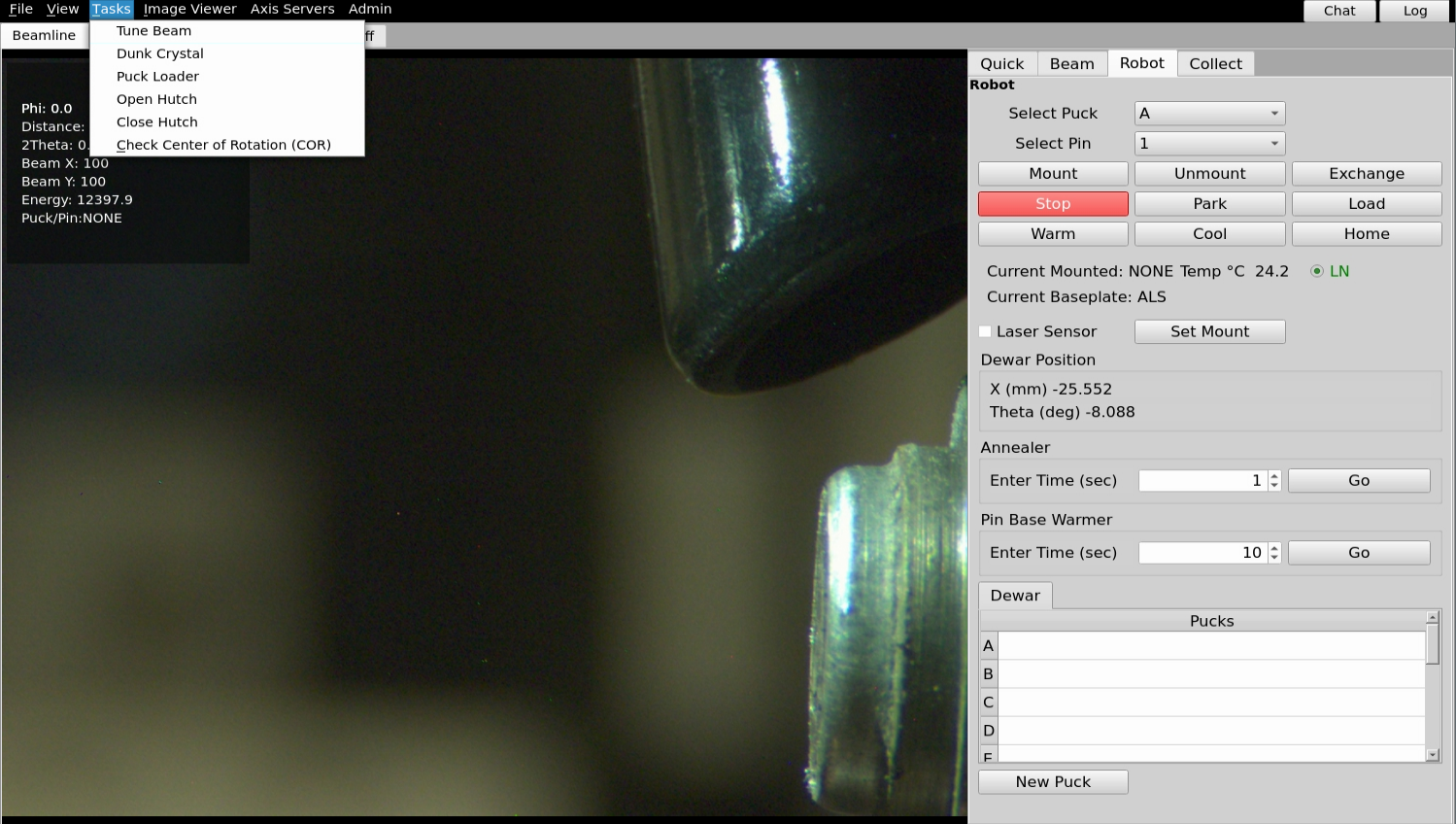
Tuning the beamline
From the Tasks pull-down menu in B4, select “Tune Beam”. This will automatically tune the monochromator and/or mirrors. The tuneup can take up to a few minutes.